Stereo Visual Odometry
Stereo Visual Odometry
Overview
In this project, I implemented stereo visual odometry using the KITTI grayscale odometry dataset. I utilized OpenCV functions and computer vision principles to estimate the motion of a vehicle based on the visual information captured by a stereo camera system.
Extracting Features
For feature extraction, I used two feature detectors, which are Scale-Invariant Feature Transform (SIFT) and Oriented FAST and Rotated BRIEF (ORB), to compare the results at the end. SIFT basically works by identifying distinctive keypoints in an image at multiple scales and orientations. It analyzes local image gradients to create scale-space representations and applies the difference of Gaussian filters to detect stable keypoints that are invariant to scale and rotation. It is often used in tasks that require accuracy, such as object recognition and image stitching.

Figure 1: Keypoints detected using SIFT
ORB combines the Features from Accelerated Segment Test (FAST) corner detection algorithm with the Binary Robust Independent Elementary Features (BRIEF) descriptor. It detects keypoints by identifying corner-like regions using intensity comparisons, and then computes binary descriptors based on pixel comparisons in predefined patches. It is favored for its efficiencies and real-time capabilities, so it is often used in SLAM and visual odometry.

Figure 2: Keypoints detected using ORB
Matching Features
For feature matching, I used the brute-force matcher, which is a straightforward approach, where each feature descriptor in one set is compared with all feature descriptors in another set. It computes the distance between descriptors and matches the descriptors based on the smallest distances. For SIFT, I used L2 norm or Euclidean distance since the descriptors are represented by real-valued vectors. For ORB, I used Hamming distance because it is designed for binary strings and is more suitable for comparing binary descriptors generated by ORB.

Figure 3: Matches found using SIFT with brute-force matching

Figure 4: Matches found using ORB with brute-force matching
Lowe’s Ratio Test
After feature matching, I used Lowe’s ratio test. For each match, it compares the distance to the nearest neighbor with the distance to the second nearest neighbor. If the ratio of these distances is below a threshold, the match is considered reliable and retained, otherwise it is discarded as ambiguous.
The way I chose this threshold was by looking at Figure 5. This tells us that the correct matches tend to be the highest around a distance ratio of 0.45, meaning that we want the distance to the closest match to be about half the distance to the second closest match in order to be certain that the feature is distinct, and not too similar to multiple features in the second image. When using ORB, I have found that a ratio of 0.6 provides the best results.
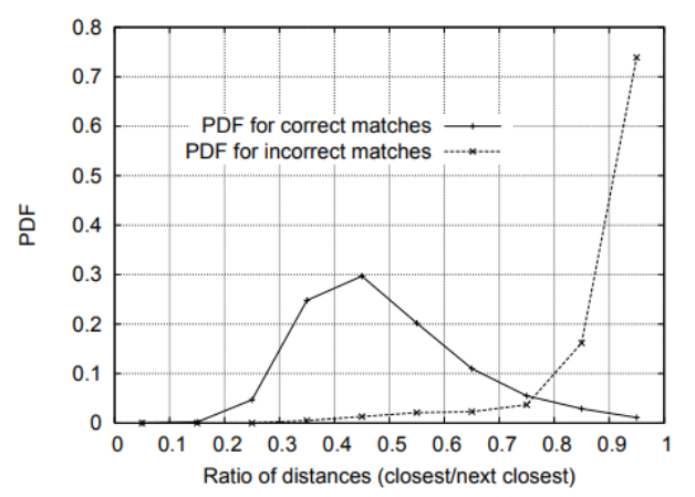
Figure 5: Probability that a match is correct based on the nearest-neighbor distance ratio test
Generating Disparity Map
The next step was to generate a disparity map. I did this by using two stereo correspondence methods, which are Stereo Block Matching (StereoBM) and Stereo Semi-Global Block Matching (StereoSGBM), to match blocks of pixels between left and right images. StereoBM basically performs a pixel-wise comparison to find the best matching block based on sum of absolute differences or sum of squared differences.

Figure 6: Disparity map generated using StereoBM
On the other hand, StereoSGBM is an extension to StereoBM and considers the consistency of disparities along different scanlines to achieve global optimization. Although it is computationally more expensive, it is able to better handle occlusions, textureless regions, and disparity discontinuities, resulting in a high-quality map.

Figure 7: Disparity map generated using StereoSGBM
Generating Depth Map
Using the disparity map computed from the previous step, we generated a depth map, which is shown below:

Figure 8: Example of a depth map
This is done by extracting the focal length from the intrinsic matrix and baseline from the translation vector, both of which are extracted from the projection matrix. Looking at Figure 9 and using similar triangles, we can derive a simple way to compute depth from the stereo pair of images if we have the baseline, focal length, and disparity.

Figure 9: Left - Diagram showing a single pixel being projected onto two different image planes. Right - Equation for calculating depth.
Estimating Motion
Using the depth map and the matched features, we can estimate the motion of the camera between two subsequent frames. We first extract the optical center of the image and the focal length from the intrinsic matrix. We then use the equations below for calculating 3D coordinates from pixel coordinates of the matched features.
![]()
Figure 10: Equations for calculating 3D coordinates
Where (u, v) represents the pixel coordinates, (c_x, c_y) represents the optical center of the image, z represents the depth, and (f_x, f_y) represents the focal length. Note that the z-coordinate in the 3D space is just the depth. The 3D points, 2D image points, and the intrinsic parameters are passed into a PnP RANSAC function in OpenCV to estimate the rotation matrix and the translation vector of the camera between two subsequent frames.
Results for KITTI Dataset Scene 9
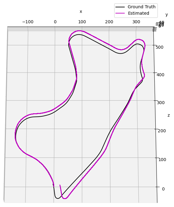
Figure 11: Plot showing the ground truth path and the estimated path after performing stereo visual odometry using SIFT
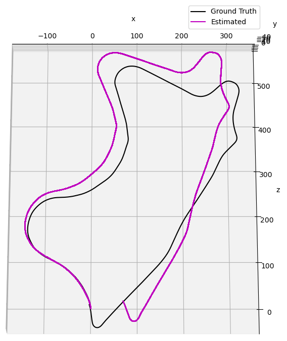
Figure 12: Plot showing the ground truth path and the estimated path after performing stereo visual odometry using ORB
When comparing the processing time of different methods, it is observed that the ground truth takes 2 minutes and 45 seconds. However, using ORB feature extraction with the Brute-Force matcher and a distance ratio of 0.6 in combination with the StereoBM algorithm, the computation time increases significantly to 5 minutes and 50 seconds. On the other hand, when employing SIFT feature extraction with the Brute-Force matcher and a distance ratio of 0.45 along with the StereoSGBM algorithm, the processing time further extends to 10 minutes and 35 seconds. Therefore, it can be concluded that ORB is approximately 55% more efficient than SIFT in terms of processing time.
When comparing the 2D endpoint accuracy of different methods, the ground truth coordinates are measured to be [-1, 8] meters, where the first number represents the x position and the second number represents the z position (as reflected in the figures above). Using ORB feature extraction, the estimated coordinates are found to be [65, 8] meters, while SIFT feature extraction yields estimated coordinates of [2, 10] meters. It is evident that SIFT is significantly closer to the ground truth, with a Euclidean distance that is 94.5% smaller than that of ORB. This indicates that SIFT provides a more accurate estimation of the 2D endpoint coordinates compared to ORB.